Explaining MLE and MAP machine learning principles visually for a newbie

3 min readOct 16, 2020

In order to estimate probabilities from data, we first make assumption about type of probability distribution from which we have sampled training data e.g. in case of coin toss, we make the assumption that coin tosses follow binomial distribution and then try to estimate the parameters of distribution using MLE/MAP estimates.

In this blog I will explain both of these estimation principles by taking coin toss example and working demo using jupyter notebook.

Here is the github link for notebook to run various simulations explained in this blog:-

https://github.com/snji-khjuria/machine_learning_abc/blob/master/notebooks/MLE-MAP%20demo.ipynb

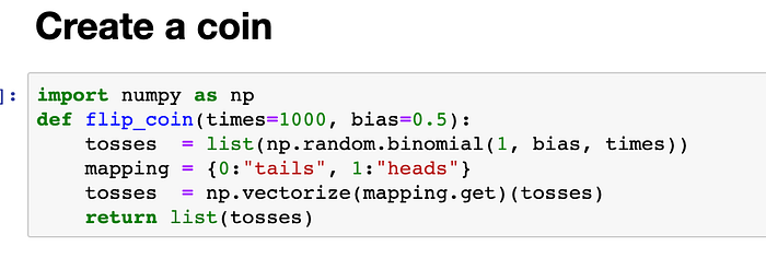
Step-1: Simulate coin toss

Step-2: Maximum likelihood estimation for sequence of tosses

Step-3 (Plot MLE Estimates): We simulate 7000 coin tosses with theta=0.6. We see that initially MLE estimates have a lot of variance because of cold start but with time, model becomes stable and reaches close to ground truth i.e. 0.6

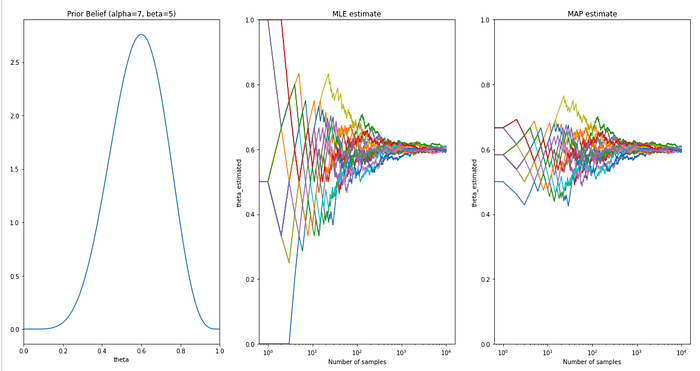
Step-4 (Plot MLE estimates from multiple experiment): In this step we will simulate 20 experiments from 20 different coins and see the MLE estimation process.

MLE has high variance initially and with time MLE estimates become more stable

Step-5: Maximum-A-Posteriori Estimation process

Step-6 (Plot MAP estimates): In this step, we guide the model by giving prior belief of 0.6 to estimation process and we can see that the MAP estimation of parameter theta remains ~0.6 throughout the estimation process for different samples of tosses of same coin.

Step-7: MLE vs. MAP estimation

a. Un-informed prior

MLE and MAP estimates remain same because no prior knowledge is given to model

b. General Prior (theta~0.5)

MAP estimate doesn’t jump here and there….stays close to 0.5 during initial samples

c. General Prior with more confidence: We are feeding-in the confidence that my coin has 0.5 probability of heads and we have observed this by flipping the coin 200 times.

References

http://www.cs.cornell.edu/courses/cs4780/2018fa/lectures/lecturenote06.html